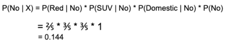
Naive Bayes classifier#
A Naive Bayes classifier is a type of probabilistic machine learning model commonly used for sorting things into different groups.
It’s especially popular in tasks involving understanding human language (like in natural language processing or text classification), identifying spam in emails, figuring out the sentiment behind a piece of text, and more.
The model relies on a statistical concept called Bayes’ theorem and makes a “naive” assumption that the different characteristics we’re looking at are independent of each other. Despite this oversimplification, Naive Bayes often turns out to be surprisingly effective in real-world situations.
Bayes’ Theorem.
Bayes’ theorem is also known as Bayes’ Rule or Bayes’ law, which is used to determine the probability of a hypothesis with prior knowledge. It depends on the conditional probability.
Conditional probability is a measure of the probability of an event occurring given that another event has (by assumption, presumption, assertion, or evidence) occurred.
The formula for Bayes’ theorem is given as:
Where:
\(P(y|X)\) is the probability of class y given the features X;
\(P(X|y)\) is the likelihood, the probability of observing features X given class y;
\(P(y)\) is the prior probability of class y;
\(P(X)\) is the evidence, the probability of observing the features X.
Conditional Independence
The “naive” assumption made by Naive Bayes is that all features are conditionally independent given the class label. In other words, the presence or absence of one feature does not affect the presence or absence of any other feature. This simplifies the calculation of the likelihood, making the model computationally tractable.
Assumptions Made by Naive Bayes#
The fundamental Naïve Bayes assumption is that each feature makes an:
independent
equal contribution to the outcome.
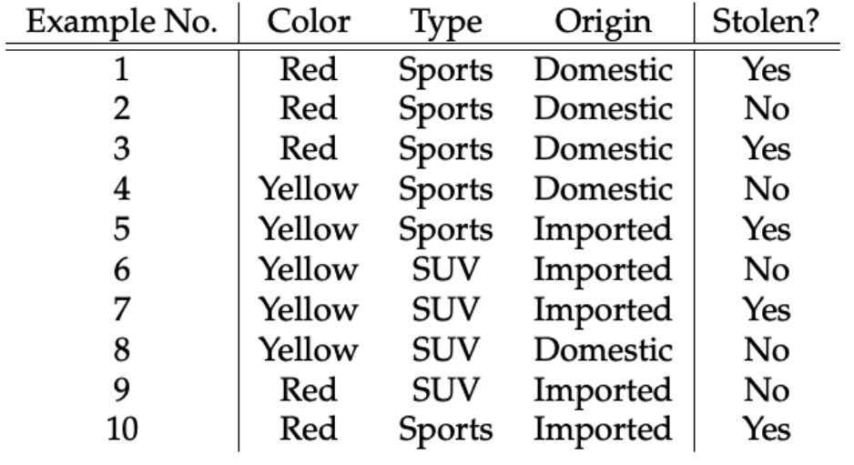
Let us take an example to get some better intuition. Consider the car theft problem with attributes Color, Type, Origin, and the target, Stolen can be either Yes or No.
Naive Bayes Example#
The dataset is represented as below:
The concept of assumptions made by the algorithm can be understood as:
We assume that no pair of features are dependent. For example, the color being ‘Red’ has nothing to do with the Type or the Origin of the car. Hence, the features are assumed to be Independent.
Secondly, each feature is given the same influence(or importance). For example, knowing the only Color and Type alone can’t predict the outcome perfectly. So none of the attributes are irrelevant and assumed to be contributing Equally to the outcome.
Note: The assumptions made by Naïve Bayes are generally not correct in real-world situations. The independence assumption is never correct but often works well in practice. Hence the name ‘Naï>ve’.
Here in our dataset, we need to classify whether the car is stolen, given the features of the car.
The columns represent these features and the rows represent individual entries. If we take the first row of the dataset, we can observe that the car is stolen if the Color is Red, the Type is Sports and Origin is Domestic. So we want to classify a Red Domestic SUV is getting stolen or not.
Let’s create tables of relative frequencies for each parameter relative to the desired result:

Frequency and Likelihood tables of ‘Color’
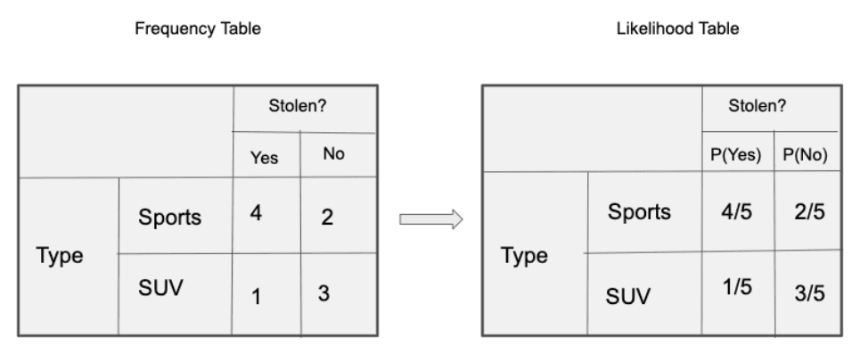
Frequency and Likelihood tables of ‘Type’
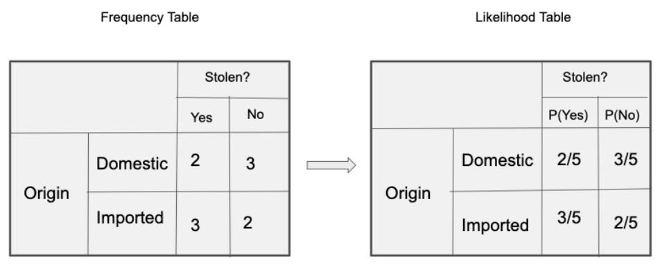
Frequency and Likelihood tables of ‘Origin’
So in our example, we have 3 predictors X.
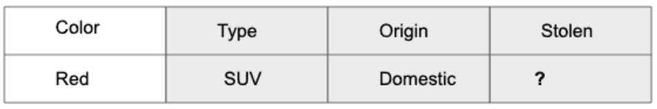
As per the equations discussed above, we can calculate the posterior probability P(Yes | X) as :
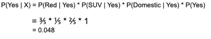
and, P( No | X ):
Since 0.144 > 0.048, Which means given the features RED SUV and Domestic, our example gets classified as ’NO’ the car is not stolen.
Types of Naive Bayes Classifiers#
Multinomial Naive Bayes.
Multinomial naive Bayes Feature vectors represent the frequencies with which certain events have been generated by a. This is the event model typically used for document classification.
Gaussian Naive Bayes.
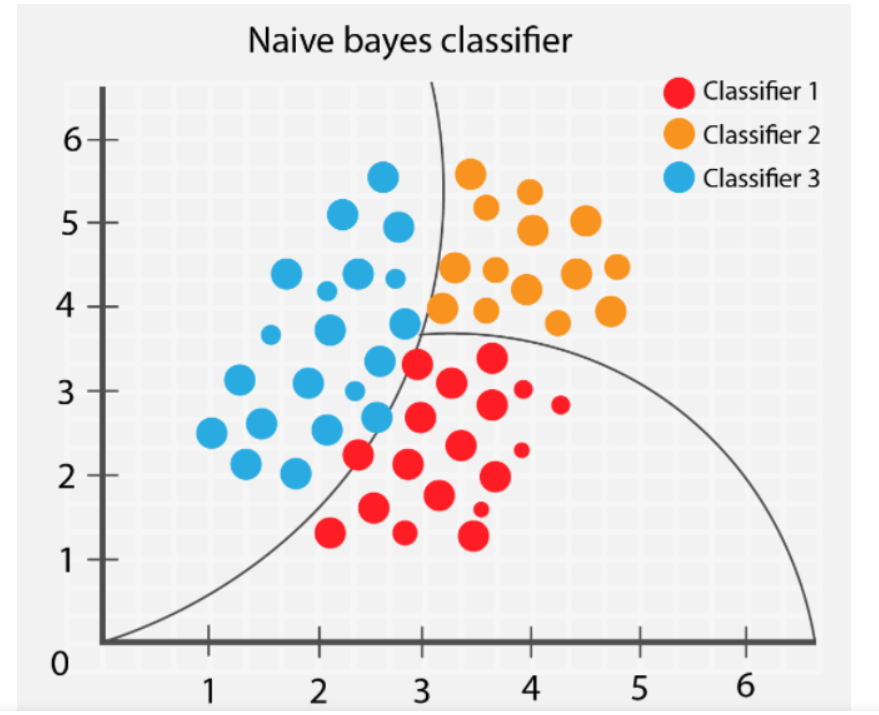
In the context of Gaussian Naive Bayes, it is assumed that the continuous values linked to each feature follow a Gaussian distribution, which is commonly referred to as a Normal distribution.
Bernoulli Naive Bayes.
In the multivariate Bernoulli event model, characteristics consist of independent boolean values (binary variables) that describe inputs. Similar to the multinomial model, this approach is well-known for tasks such as document classification, specifically focusing on the occurrence of binary terms.
Advantages
Simplicity and speed: Naive Bayes is computationally efficient and can handle high-dimensional data;
Works well with small datasets;
Often performs surprisingly well, especially in text classification tasks;
Provides probabilities, allowing for probabilistic predictions.
Limitations
The “naive” assumption of feature independence may not hold in many real-world scenarios;
If the features are highly correlated, Naive Bayes may produce suboptimal results.
It doesn’t handle missing data well.
Naive Bayes classifiers are widely used as a baseline model in many classification problems due to their simplicity and effectiveness, especially when working with text data. However, they may not be the best choice for every problem, and more complex models like decision trees, random forests, or neural networks may provide better accuracy in some cases.
Approaches to classification training: Discriminative vs generative models#
Generative Approach: Models how data can be generated for each class. For example, it estimates the probabilities of the occurrence of each word in a document for spam and non-spam classes.
Discriminative Approach: Focuses on directly discerning between classes. For instance, it estimates the probability that an email is spam based on a set of features.
Discriminative models are often preferred when the emphasis is on classification accuracy, and there’s less concern about generating new samples
A discriminative model learns posterior distribution \(p(y \vert \boldsymbol x, \boldsymbol w)\). Example: logistic regression model
Generative models are useful when the goal is to generate new samples or when dealing with missing data. They also have applications in unsupervised learning.
A generative model estimates joint distribution
Bayesian classifier#
For classification use Bayes theorem:
Bayesian classifier maximizes this expression:
How to estimate \(\mathbb P(y = k)\) and \(p(\boldsymbol x \vert y = k)\) given a training dataset \((\boldsymbol X, \boldsymbol y)\)?
In Gaussian Naïve Bayes, continuous values associated with each feature are assumed to be distributed according to a Gaussian distribution (Normal distribution). When plotted, it gives a bell-shaped curve which is symmetric about the mean of the feature values as shown below:
Special cases of parametric density estimation:
Quadratic discriminant analysis (QDA): allows for different covariance matrices for each class, making it more flexible in capturing the underlying structure of the data.
Linear discriminant analysis (LDA): the covariance matrix \(\boldsymbol \Sigma\) is the same for all classes, and it’s MLE estimation is
Naive Bayes estimation#
Naive assumption: refers to treating features as if they are independent given the class label, simplifying the modeling process. All feature, conditioned on target, are independent:
To estimate 1-d densities \(p(x_j \vert y)\) is much easier than multivariate ones. The output of the Bayesian classifier is given by
Python implementations of the models#
Multinomial Naive Bayes#
Here’s an example of how to implement a Multinomial Naive Bayes classifier in Python using scikit-learn. In this example, we’ll use the famous “20 Newsgroups” dataset for text classification, where the task is to classify news articles into one of 20 different categories.
from sklearn.datasets import fetch_20newsgroups
from sklearn.feature_extraction.text import CountVectorizer, TfidfTransformer
from sklearn.naive_bayes import MultinomialNB
from sklearn.pipeline import Pipeline
from sklearn.model_selection import train_test_split
from sklearn import metrics

# Load the 20 Newsgroups dataset
newsgroups = fetch_20newsgroups(subset='all', remove=('headers', 'footers', 'quotes'))

# Split the dataset into training and testing sets
X_train, X_test, y_train, y_test = train_test_split(newsgroups.data, newsgroups.target, test_size=0.25, random_state=42)

# Create a pipeline for text classification with Multinomial Naive Bayes
text_clf = Pipeline([
    ('vect', CountVectorizer()),  # Convert text to a bag-of-words representation
    ('tfidf', TfidfTransformer()),  # Convert raw frequency counts to TF-IDF values
    ('clf', MultinomialNB())  # Multinomial Naive Bayes classifier
])

# Fit the model on the training data
text_clf.fit(X_train, y_train)

# Make predictions on the test data
y_pred = text_clf.predict(X_test)

# Evaluate the model
accuracy = metrics.accuracy_score(y_test, y_pred)
print(f"Accuracy: {accuracy:.2f}")
Accuracy: 0.65
In this code:
We load the 20 Newsgroups dataset and split it into training and testing sets.
We create a pipeline for text classification, which includes text preprocessing steps like converting text to a bag-of-words representation and then to TF-IDF (Term Frequency-Inverse Document Frequency) values.
We use the Multinomial Naive Bayes classifier from scikit-learn (MultinomialNB) as the final step in the pipeline.
We fit the model on the training data and make predictions on the test data.
Finally, the accuracy of the model is evaluated using scikit-learn’s accuracy_score function.
Gaussian Naive Bayes classifier#
Here’s an example of how to implement a Gaussian Naive Bayes classifier in Python using scikit-learn. Gaussian Naive Bayes is typically used for classification problems where the features are continuous and assumed to follow a Gaussian (normal) distribution.
In this example, we’ll use a commonly used dataset for classification tasks:
from sklearn.datasets import load_breast_cancer
from sklearn.model_selection import train_test_split
from sklearn.naive_bayes import GaussianNB
from sklearn import metrics

# Load the Breast Cancer dataset
cancer = load_breast_cancer()
X = cancer.data
y = cancer.target

# Split the dataset into training and testing sets
X_train, X_test, y_train, y_test = train_test_split(X, y, test_size=0.25, random_state=42)

gnb = GaussianNB()

gnb.fit(X_train, y_train)

y_pred = gnb.predict(X_test)

accuracy = metrics.accuracy_score(y_test, y_pred)
print(f"Accuracy: {accuracy:.2f}")
Accuracy: 0.96
In this code:
The Breast Cancer dataset is loaded using load_breast_cancer from scikit-learn’s datasets.
The dataset is split into training and testing sets using train_test_split.
A Gaussian Naive Bayes classifier (GaussianNB) is instantiated.
The classifier is trained on the training data using the fit method.
Predictions are made on the test data using the predict method.
This example uses the Gaussian Naive Bayes classifier to predict whether a tumor is malignant or benign based on features such as mean radius, mean texture, mean smoothness, etc.
Bernoulli Naive Bayes classifier#
Here’s an example of how to implement a Bernoulli Naive Bayes classifier in Python using scikit-learn. Bernoulli Naive Bayes is typically used for binary classification tasks where features are binary, representing the presence or absence of certain attributes.
In this example, we’ll use a synthetic dataset for binary classification:
from sklearn.datasets import make_classification
from sklearn.model_selection import train_test_split
from sklearn.naive_bayes import BernoulliNB
from sklearn import metrics

X, y = make_classification(n_samples=1000, n_features=20, random_state=42)

# Split the dataset into training and testing sets
X_train, X_test, y_train, y_test = train_test_split(X, y, test_size=0.3, random_state=42)

bnb = BernoulliNB()

bnb.fit(X_train, y_train)

y_pred = bnb.predict(X_test)

accuracy = metrics.accuracy_score(y_test, y_pred)
print(f"Accuracy: {accuracy:.2f}")
Accuracy: 0.80
In this code:
A synthetic binary classification dataset is generated using the make_classification function from scikit-learn.
The dataset is divided into training and testing sets.
A Bernoulli Naive Bayes classifier is instantiated using the BernoulliNB class.
The model is trained on the provided training data.
Predictions are made on the test data, and the accuracy of the model is assessed.
This illustration showcases the application of Bernoulli Naive Bayes for solving a binary classification problem with binary features.
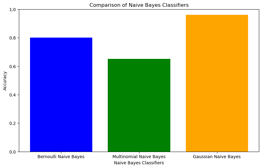
import matplotlib.pyplot as plt
import numpy as np

classifiers = ['Bernoulli Naive Bayes', 'Multinomial Naive Bayes', 'Gaussian Naive Bayes']
accuracy = [0.80, 0.65, 0.96]

# Строим столбчатую диаграмму для сравнения точности классификаторов.
plt.figure(figsize=(10, 6))
plt.bar(classifiers, accuracy, color=['blue', 'green', 'orange'])
plt.ylim(0, 1)
plt.title('Comparison of Naive Bayes Classifiers')
plt.xlabel('Naive Bayes Classifiers')
plt.ylabel('Accuracy')
plt.show()
from jupyterquiz import display_quiz
def get_spanned_encoded_q(q, q_name):
    byte_code = b64encode(bytes(json.dumps(q), 'utf8'))
    return f'<span style="display:none" id="{q_name}">{byte_code.decode()}</span>'
from IPython.display import HTML

HTML('''<script>
code_show=true;
function code_toggle() {
 if (code_show){
 $('div.input').hide();
 } else {
 $('div.input').show();
 }
 code_show = !code_show
}
$( document ).ready(code_toggle);
</script>
<form action="javascript:code_toggle()"><input type="submit" value="Click here to toggle on/off the raw code."></form>''')
q_b_a = [{
    "question": "In what scenarios might it be most appropriate to use the Naive Bayes classifier considering its principles and assumptions?",
    "type": "many_choice",
    "answers": [
        {
            "answer": "When features are strongly correlated and dependent on each other",
            "correct": False,
            "feedback": "Incorrect"
        },
        {
            "answer": "In tasks where the data contains a large number of numerical features",
            "correct": False,
            "feedback": "Incorrect"
        },
        {
            "answer": "When the assumption of independence among features is more critical to the end result",
            "correct": False,
            "feedback": "Incorrect"
        },
        {
            "answer": "In tasks involving the classification of textual data, such as sentiment analysis of reviews",
            "correct": True,
            "feedback": "Correct"
        },
    ]
}]
display_quiz(q_b_a)
from IPython.display import HTML

HTML('''<script>
code_show=true;
function code_toggle() {
 if (code_show){
 $('div.input').hide();
 } else {
 $('div.input').show();
 }
 code_show = !code_show
}
$( document ).ready(code_toggle);
</script>
<form action="javascript:code_toggle()"><input type="submit" value="Click here to toggle on/off the raw code."></form>''')
q_b_b = [{
    "question": "How does a Naive Bayes classifier calculate the probability of an event, and what are the key steps involved in this process?",
    "type": "many_choice",
    "answers": [
        {
            "answer": "It relies on deep learning techniques exclusively",
            "correct": False,
            "feedback": "Incorrect"
        },
        {
            "answer": "It estimates probabilities for informed classification",
            "correct": True,
            "feedback": "Correct"
        },
        {
            "answer": "It uses unsupervised learning for probability estimation",
            "correct": False,
            "feedback": "Incorrect"
        },
        {
            "answer": "It ignores probability calculations and relies solely on feature independence",
            "correct": False,
            "feedback": "Incorrect"
        },
    ]
}]
display_quiz(q_b_b)
Example: Titanic#
import numpy as np
import pandas as pd
import matplotlib.pyplot as plt
import seaborn as sns
import warnings
warnings.filterwarnings('ignore')
%matplotlib inline
The data has been split into two groups:
training set (train.csv) test set (test.csv) The training set should be used to build your machine learning models. For the training set, we provide the outcome (also known as the “ground truth”) for each passenger. Our model will be based on “features” like passengers’ gender and class. We also will use feature engineering to create new features.
train_df=pd.read_csv("train.csv")
test_df=pd.read_csv("test.csv")
train_df.head()
| PassengerId | Survived | Pclass | Name | Sex | Age | SibSp | Parch | Ticket | Fare | Cabin | Embarked | |
|---|---|---|---|---|---|---|---|---|---|---|---|---|
| 0 | 1 | 0 | 3 | Braund, Mr. Owen Harris | male | 22.0 | 1 | 0 | A/5 21171 | 7.2500 | NaN | S |
| 1 | 2 | 1 | 1 | Cumings, Mrs. John Bradley (Florence Briggs Th... | female | 38.0 | 1 | 0 | PC 17599 | 71.2833 | C85 | C |
| 2 | 3 | 1 | 3 | Heikkinen, Miss. Laina | female | 26.0 | 0 | 0 | STON/O2. 3101282 | 7.9250 | NaN | S |
| 3 | 4 | 1 | 1 | Futrelle, Mrs. Jacques Heath (Lily May Peel) | female | 35.0 | 1 | 0 | 113803 | 53.1000 | C123 | S |
| 4 | 5 | 0 | 3 | Allen, Mr. William Henry | male | 35.0 | 0 | 0 | 373450 | 8.0500 | NaN | S |
test_df['Age'].mean()
train_df['Embarked'].fillna(train_df['Embarked'].mode()[0], inplace = True)
test_df['Fare'].fillna(test_df['Fare'].median(), inplace = True)
drop_column = ['Cabin']
train_df.drop(drop_column, axis=1, inplace = True)
test_df.drop(drop_column,axis=1,inplace=True)
test_df['Age'].fillna(test_df['Age'].median(), inplace = True)
train_df['Age'].fillna(train_df['Age'].median(), inplace = True)
Some feature engineering, adjusting the code.
We will use just two techniques:
Polynomials generation through non-linear expansions and Box-Cox transformations. But for now we will adjust data
all_data=[train_df,test_df]
for dataset in all_data:
    dataset['FamilySize'] = dataset['SibSp'] + dataset['Parch'] + 1
import re
# Define function to extract titles from passenger names
def get_title(name):
    title_search = re.search(' ([A-Za-z]+)\.', name)
    # If the title exists, extract and return it.
    if title_search:
        return title_search.group(1)
    return ""
# Create a new feature Title, containing the titles of passenger names
for dataset in all_data:
    dataset['Title'] = dataset['Name'].apply(get_title)
# Group all non-common titles into one single grouping "Rare"
for dataset in all_data:
    dataset['Title'] = dataset['Title'].replace(['Lady', 'Countess','Capt', 'Col','Don',
                                                 'Dr', 'Major', 'Rev', 'Sir', 'Jonkheer', 'Dona'], 'Rare')

    dataset['Title'] = dataset['Title'].replace('Mlle', 'Miss')
    dataset['Title'] = dataset['Title'].replace('Ms', 'Miss')
    dataset['Title'] = dataset['Title'].replace('Mme', 'Mrs')
for dataset in all_data:
    dataset['Age_bin'] = pd.cut(dataset['Age'], bins=[0,12,20,40,120], labels=['Children','Teenage','Adult','Elder'])
for dataset in all_data:
    dataset['Fare_bin'] = pd.cut(dataset['Fare'], bins=[0,7.91,14.45,31,120], labels=['Low_fare','median_fare',
                                                                                      'Average_fare','high_fare'])
all_dat=[train_df,test_df]
for dataset in all_dat:
    drop_column = ['Age','Fare','Name','Ticket']
    dataset.drop(drop_column, axis=1, inplace = True)
drop_column = ['PassengerId']
train_df.drop(drop_column, axis=1, inplace = True)
Now we converte the catergical features in numerical by using dummy variable
traindf = pd.get_dummies(train_df, columns = ["Sex","Title","Age_bin","Embarked","Fare_bin"],
                             prefix=["Sex","Title","Age_type","Em_type","Fare_type"])
testdf = pd.get_dummies(test_df, columns = ["Sex","Title","Age_bin","Embarked","Fare_bin"],
                             prefix=["Sex","Title","Age_type","Em_type","Fare_type"])
Now we are ready to train a model and predict the required solution. We want to identify relationship between output (Survived or not) with other variables or features (Gender, Age, Port, etc.), so we are using supervised model of Naive Bayes.
from sklearn.model_selection import train_test_split #for split the data
from sklearn.metrics import accuracy_score  #for accuracy_score
from sklearn.model_selection import KFold #for K-fold cross validation
from sklearn.model_selection import cross_val_score #score evaluation
from sklearn.model_selection import cross_val_predict #prediction
from sklearn.metrics import confusion_matrix #for confusion matrix
all_features = traindf.drop("Survived",axis=1)
Targeted_feature = traindf["Survived"]
X_train,X_test,y_train,y_test = train_test_split(all_features,Targeted_feature,test_size=0.3,random_state=42)
X_train.shape,X_test.shape,y_train.shape,y_test.shape
((623, 22), (268, 22), (623,), (268,))
# Gaussian Naive Bayes
from sklearn.naive_bayes import GaussianNB
model= GaussianNB()
model.fit(X_train,y_train)
prediction_gnb=model.predict(X_test)
print('--------------The Accuracy of the model----------------------------')
print('The accuracy of the Gaussian Naive Bayes Classifier is',round(accuracy_score(prediction_gnb,y_test)*100,2))
kfold = KFold(n_splits=10, random_state=22, shuffle=True) # k=10, split the data into 10 equal parts
result_gnb=cross_val_score(model,all_features,Targeted_feature,cv=10,scoring='accuracy')
print('The cross validated score for Gaussian Naive Bayes classifier is:',round(result_gnb.mean()*100,2))
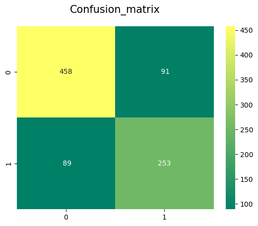
y_pred = cross_val_predict(model,all_features,Targeted_feature,cv=10)
sns.heatmap(confusion_matrix(Targeted_feature,y_pred),annot=True,fmt='3.0f',cmap="summer")
plt.title('Confusion_matrix', y=1.05, size=15)
--------------The Accuracy of the model----------------------------
The accuracy of the Gaussian Naive Bayes Classifier is 79.48
The cross validated score for Gaussian Naive Bayes classifier is: 79.8
Text(0.5, 1.05, 'Confusion_matrix')
from IPython.display import HTML

HTML('''<script>
code_show=true;
function code_toggle() {
 if (code_show){
 $('div.input').hide();
 } else {
 $('div.input').show();
 }
 code_show = !code_show
}
$( document ).ready(code_toggle);
</script>
<form action="javascript:code_toggle()"><input type="submit" value="Click here to toggle on/off the raw code."></form>''')
q_b_c = [{
    "question": "What is a key advantage of the Naive Bayes classifier in scenarios with limited data compared to other complex models?",
    "type": "many_choice",
    "answers": [
        {
            "answer": "It requires a large amount of labeled training data for accurate predictions",
            "correct": False,
            "feedback": "Incorrect"
        },
        {
            "answer": "It tends to overfit the training data easily",
            "correct": False,
            "feedback": "Incorrect"
        },
        {
            "answer": "It performs well only when there is a high degree of correlation among features",
            "correct": False,
            "feedback": "Incorrect"
        },
        {
            "answer": "Its simplicity and assumption of feature independence reduce overfitting in limited data situations",
            "correct": True,
            "feedback": "Correct"
        },
    ]
}]
display_quiz(q_b_c)